Usage
Quick Explanation
The example below shows how to use planetaryimage‘s PDS3Image class to
open a PDS image, inspect it’s label and display the image data:
>>> from planetaryimage import PDS3Image
>>> import matplotlib.pyplot as plt
>>> testfile = 'tests/mission_data/2p129641989eth0361p2600r8m1.img'
>>> image = PDS3Image.open(testfile)
>>> print(image.record_bytes)               # access attribute
128
>>> print(image.label['FILE_RECORDS'])      # access label
332
>>> plt.imshow(image.image, cmap='gray')  # display image
Examples
Setup:
>>> %matplotlib inline
>>> from glob import glob
>>> import numpy as np
>>> import matplotlib.pyplot as plt
>>> import matplotlib.image as mpimg
>>> from planetaryimage import PDS3Image, CubeFile
Gather the Images:
>>> pdsfiles = glob("*.*")
>>> images = []
>>> for pdsfile in pdsfiles:
...    try:
...        images.append(PDS3Image.open(pdsfile))
...    except:
...        pass
>>> for n, image in enumerate(images):
...    print n, image
0 1p190678905erp64kcp2600l8c1.img
1 mk19s259.img
2 m0002320.imq
3 mg00n217.sgr
4 h2225_0000_dt4.img
5 0044ML0205000000E1_DXXX.img
One can use the try statement in-case any of the images you have are
not compatible with PDS3image. See Suppored Planetary Images List
to know what image types are compatible. The for loop will show what index
number to use in future use of the image.
To see the information about each image:
>>> for i in images:
...    print i.data.dtype, i.data.shape, i.shape
>i2 (1, 1024, 32) (1, 1024, 32)
uint8 (1, 1331, 1328) (1, 1331, 1328)
uint8 (1, 1600, 384) (1, 1600, 384)
uint8 (1, 960, 964) (1, 960, 964)
>i2 (1, 10200, 1658) (1, 10200, 1658)
uint8 (3, 1200, 1648) (3, 1200, 1648)
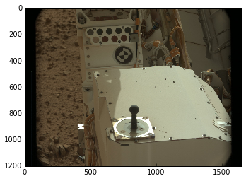
To display a three band, color, image:
>>> caltarget = images[5]
>>> plt.imshow(caltarget.image)
<matplotlib.image.AxesImage at 0x10a13c250>
It is important to look at the first number in i.shape (See attributes) or
the value from i.bands. If this number is 3, then the above example works,
otherwise, you should use cmap=='gray' parameter like in the below example.
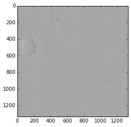
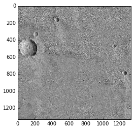
To display a single band, grayscale, image:
>>> image1 = images[1]
>>> plt.imshow(image1.image, cmap='gray')
<matplotlib.image.AxesImage at 0x125817a50>
The cmap keyword argument defines which colormap a grayscale image
should be displayed with. In the case where i.bands is 3, it means the
image is an RGB color image which does not need a colormap to be displayed
properly. If i.bands is 1, then the image is grayscale and imshow
would use its default colormap, which is not grayscale.
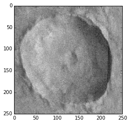
To see a subframe of an image:
>>> plt.imshow(image1.image[370:620, 0:250], cmap = 'gray')
<matplotlib.image.AxesImage at 0x11c014450>
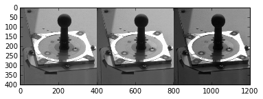
To see the different bands of a colored image:
>>> plt.imshow(np.hstack([
       mcam1.image[700:1100, 600:1000, 0],
       mcam1.image[700:1100, 600:1000, 1],
       mcam1.image[700:1100, 600:1000, 2],
   ]), cmap='gray')
<matplotlib.image.AxesImage at 0x10fccd210>
To save an image as a .png file for later viewing:
>>> crater = image1.image[370:620, 0:250]
>>> plt.imsave('crater.png', crater, cmap='gray')
To do some image processing:
>>> plt.hist(image1.image.flatten(), 2000)
(array([ 2.,  0.,  0., ...,  0.,  0.,  1.]),
array([  32.   ,   32.036,   32.072, ...,  175.928,  175.964,  176.   ]),
<a list of 4000 Patch objects>)
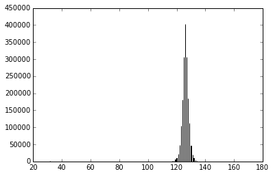
Using this Histogram can produce a clearer picture:
>>> plt.imshow(image1.image, cmap='gray', vmin=115, vmax=135)
<matplotlib.image.AxesImage at 0x1397a2790>
See documentation for plt.imshow and Image tutorial for pyplot to see more methods of image processing.
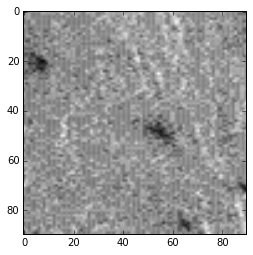
You can also use planetaryimage to process Isis Cube Files:
>>> from planetaryimage import CubeFile
>>> isisimage = CubeFile.open("tests/data/pattern.cub")
>>> isisimage.data.dtype, isisimage.data.shape, isisimage.shape
(dtype('<f4'), (90, 90), (1, 90, 90))
>>> plt.imshow(isisimage.image, cmap='gray')
<matplotlib.image.AxesImage at 0x114010610>